Research Study

EEG-Based State Classification

"How do preprocessing pipelines, regularization strategies, and class-imbalance handling interact to affect logistic regression performance on EEG datasets with varying characteristics?"

3 EEG Datasets

547 Data Files

5 Hypotheses Tested

10 Result Tables

3 Pipelines (A, B, C)

Total Error = Bias² + Variance + Noise

The fundamental bias-variance decomposition guiding all regularization and pipeline design decisions in this study.

3

Datasets

UCI Seizure · Bonn EEG · Eye State

547

Data Files

Across all three datasets

0.811

Best PR-AUC

Bonn EEG · Pipeline A

Pipe A + L2

Best Config

C=1 · Bonn EEG dataset

5

Hypotheses

H1–H5 · Kruskal-Wallis / Mann-Whitney

10

Result Tables

Holdout · Baseline · Reg · Imbalance

Dataset Summary

Three EEG datasets with distinct characteristics, class distributions, and classification challenges.

UCI Seizure

Seizure Detection

11,500

Samples

178

Features

1:4

Class Ratio

0.452

Holdout PR-AUC

Seizure class (minority)

Non-seizure (majority)

Bonn EEG

Ictal vs Non-Ictal

500

Samples

6

Features (eng.)

mild

Imbalance

0.811

Holdout PR-AUC

Ictal (seizure) class

Non-ictal class

EEG Eye State

Eye Open / Closed

14,980

Samples

14

Features

~45:55

Class Ratio

0.593

Holdout PR-AUC

Eye closed (class 1)

Eye open (class 0)

Experiment Architecture

End-to-end workflow from raw EEG data to final evaluation metrics.

Raw EEG Data

Preprocessing

Imbalance Handling

LogReg + Regularization

Evaluation

Results

PREPROCESSING

Pipeline A: StandardScaler + MI SelectKBest(k=20)
Pipeline B: StandardScaler + PCA(95%)
Pipeline C: Wavelet + StandardScaler + PCA(95%)

REGULARIZATION

L1 (Lasso) · L2 (Ridge) · ElasticNet (α=0.5)
C values: 0.001, 0.01, 0.1, 1, 10, 100
Cross-validated on training set

IMBALANCE

SMOTE oversampling
Random undersampling
Class weight balancing

EVALUATION

PR-AUC (primary metric)
F1, Recall, Precision, Accuracy
Kruskal-Wallis & Mann-Whitney tests

Hypothesis Overview

Five statistical hypotheses tested using non-parametric tests (α = 0.05).

H1 Partial

Pipeline Effect on Performance

Does preprocessing pipeline choice significantly affect PR-AUC across datasets?

UCI p=0.166 (n.s.) · Eye State p=0.000082 ✓

H2 Not Sig.

Regularization Generalization

Does regularization type (L1/L2/EN) significantly affect holdout PR-AUC?

L1 vs L2 p=0.914 · L1 vs EN p=0.698 · L2 vs EN p=0.769

H3 Not Sig.

ElasticNet Advantage

Does ElasticNet outperform pure L1/L2 regularization on Bonn EEG?

L1 vs L2 p=0.380 · L1 vs EN p=0.544 · L2 vs EN p=0.314

H4 Not Sig.

Imbalance × Regularization

Does imbalance handling method interact with regularization type?

All pairwise comparisons p > 0.2 (none significant)

H5 SIGNIFICANT

Polynomial Overfitting

Does polynomial feature expansion cause significant overfitting vs baseline?

Baseline vs Poly p=0.0000031 ★ Highly Significant

Datasets

Three EEG datasets with distinct recording conditions, feature spaces, and classification challenges.

UCI Seizure Dataset

Epileptic seizure recognition dataset from UCI ML Repository. Each sample represents a 1-second EEG segment with 178 time-domain amplitude values. The original 5-class dataset was binarized: class 1 (seizure) vs classes 2–5 (non-seizure), creating a severe 1:4 class imbalance.

11,500

Total Samples

178

Raw Features

2,300

Seizure (pos)

9,200

Non-seizure (neg)

KEY CHALLENGE

Severe class imbalance (1:4) combined with high dimensionality (178 features) makes standard accuracy misleading. PR-AUC is the primary metric.

HOLDOUT PERFORMANCE

PR-AUC: 0.452

F1: 0.043

Recall: 0.022

Precision: 1.000

Bonn EEG Dataset

University of Bonn epilepsy dataset with 5 classes (Z, O, N, F, S). Binary classification: ictal (S class) vs non-ictal (all others). Raw signals have 4097 time points per segment; engineered features reduce this to 6 statistical descriptors (mean, std, skewness, kurtosis, energy, zero-crossing rate).

500

Total Samples

6

Eng. Features

100

Ictal (pos)

400

Non-ictal (neg)

KEY CHALLENGE

Small dataset (500 samples) with only 6 features after engineering. Pipeline C (wavelet denoising) was designed specifically for this dataset's raw signal characteristics.

HOLDOUT PERFORMANCE

PR-AUC: 0.811

F1: 0.618

Recall: 0.525

Precision: 0.750

EEG Eye State Dataset

Continuous EEG recording from a single subject with eye state labels (open=0, closed=1). 14 EEG channels recorded at 128 Hz. The dataset is nearly balanced (~45:55) but exhibits strong temporal autocorrelation, making random splits potentially optimistic.

14,980

Total Samples

14

EEG Channels

~6,741

Eye closed (pos)

~8,239

Eye open (neg)

KEY CHALLENGE

Temporal autocorrelation in continuous recording. Pipeline choice has a statistically significant effect (H1: p=0.000082), with Pipeline A substantially outperforming Pipeline B.

HOLDOUT PERFORMANCE

PR-AUC: 0.593

F1: 0.442

Recall: 0.367

Precision: 0.558

Class Distribution & Feature Comparison

Visual comparison of class balance and feature dimensionality across datasets.

Class Distribution by Dataset

Feature Count Comparison

Dataset Characteristics Summary

Dataset	Samples	Raw Features	Eng. Features	Pos Class	Neg Class	Imbalance Ratio	Task	Holdout PR-AUC
UCI Seizure	11,500	178	20 (MI top-k)	2,300	9,200	1:4 (severe)	Seizure detection	0.452
Bonn EEG	500	4,097 (raw)	6 (engineered)	100	400	1:4 (mild)	Ictal vs non-ictal	0.811
EEG Eye State	14,980	14	14 (all used)	~6,741	~8,239	~45:55 (balanced)	Eye open/closed	0.593

Preprocessing Pipelines

Three preprocessing pipelines designed to evaluate different feature extraction and dimensionality reduction strategies.

Pipeline A — MI Feature Selection

Applied to: UCI Seizure, EEG Eye State

Raw Features

↓

StandardScaler

↓

MI SelectKBest (k=20)

↓

Logistic Regression

Mutual Information selects the top-k features most informative about the target class. Preserves interpretability — selected features have direct physical meaning. Best for datasets where feature relevance varies significantly.

Pipeline B — PCA Compression

Applied to: UCI Seizure, EEG Eye State

Raw Features

↓

StandardScaler

↓

PCA (95% variance)

↓

Logistic Regression

PCA retains components explaining 95% of variance. Reduces dimensionality while capturing global structure. Loses interpretability but may reduce noise. Components are linear combinations of all original features.

Pipeline C — Wavelet + PCA

Applied to: Bonn EEG only

Raw EEG Signal

↓

Wavelet Denoiser (db4)

↓

StandardScaler

↓

PCA (95% variance)

↓

Logistic Regression

Daubechies-4 wavelet denoising removes high-frequency noise before feature extraction. Designed for Bonn EEG's raw 4097-point signals. Surprisingly underperforms Pipeline A/B on this dataset (PR-AUC 0.765 vs 0.882).

Dimensionality Reduction: Input → Output Features

Dataset	Input Features	Pipeline A Output	Pipeline B Output	Pipeline C Output	Reduction (A)	Reduction (B)
UCI Seizure	178	20 (MI top-20)	~30 (PCA 95%)	N/A	88.8% reduction	~83% reduction
Bonn EEG	6 (engineered)	6 (all selected)	~5 (PCA 95%)	~5 (Wavelet+PCA)	0% reduction	~17% reduction
EEG Eye State	14	14 (all selected)	~10 (PCA 95%)	N/A	0% reduction	~29% reduction

Baseline Pipeline Results (Table 1) — PR-AUC Comparison

Pipeline	Dataset	PR-AUC	F1	Recall	Notes
Pipeline A	UCI Seizure	0.464	0.046	0.023	MI selection, 20 features
Pipeline B	UCI Seizure	0.480	0.105	0.055	PCA compression
Pipeline A	Bonn EEG	0.882	0.755	0.688	Best overall configuration
Pipeline B	Bonn EEG	0.881	0.738	0.663	Near-identical to Pipeline A
Pipeline C	Bonn EEG	0.765	0.632	0.563	Wavelet denoising underperforms
Pipeline A	EEG Eye State	0.618	0.546	0.488	MI selection dominant
Pipeline B	EEG Eye State	0.559	0.370	0.287	PCA loses discriminative info

Train/Validation Gap — C Parameter Effect

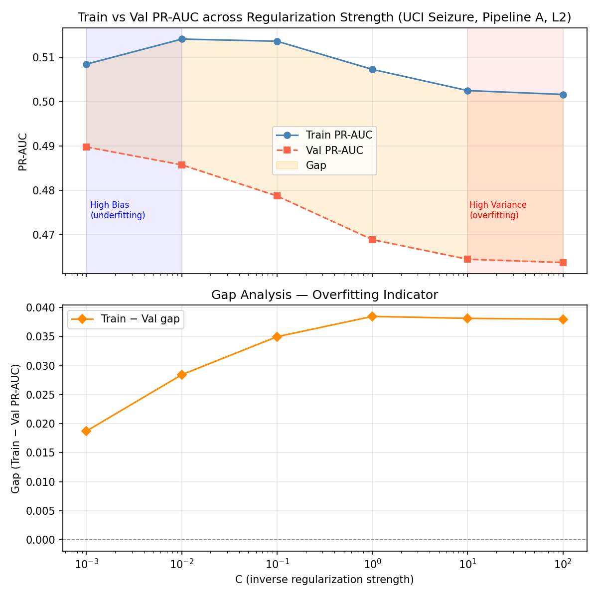
Train vs validation PR-AUC gap as a function of regularization strength C. Higher C = less regularization = potential overfitting.

Regularization Analysis

Comparing L1 (Lasso), L2 (Ridge), and ElasticNet regularization across datasets and C values.

Regularization Comparison — Pipeline A, C=1 (Best Config)

Regularization	Dataset	PR-AUC	Δ vs L2	Sparsity	Notes
L1 (Lasso)	UCI Seizure	0.470	+0.001	5/20 nonzero	Sparse solution, 75% features zeroed
L2 (Ridge)	UCI Seizure	0.469	—	20/20 nonzero	Dense solution, all features used
ElasticNet (α=0.5)	UCI Seizure	0.470	+0.001	~10/20 nonzero	Intermediate sparsity
L1 (Lasso)	Bonn EEG	0.884	+0.004	0/6 nonzero (C=0.01)	Aggressive sparsity at low C
L2 (Ridge)	Bonn EEG	0.880	—	6/6 nonzero	All features retained
L1 (Lasso)	EEG Eye State	0.604	-0.001	5/14 nonzero	Selects 5 most informative channels
L2 (Ridge)	EEG Eye State	0.605	—	14/14 nonzero	Marginal advantage over L1

H2 Finding: No statistically significant difference between L1, L2, and ElasticNet (all p > 0.69). Regularization type has minimal impact on PR-AUC when C is optimized. The choice of C (regularization strength) matters far more than the penalty type.

Sparsity: Nonzero Coefficients (C=0.01)

At C=0.01 (strong regularization), L1 aggressively zeros out coefficients while L2 retains all. Bonn EEG with L1 reaches complete sparsity (0/6 features), effectively predicting the majority class.

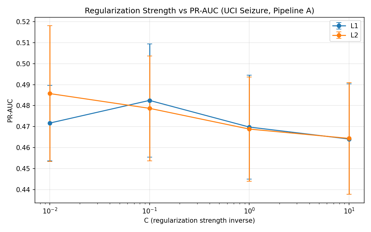
PR-AUC vs C Value (Pipeline A, L1 vs L2)

Performance peaks around C=1 for most datasets. Very low C (strong regularization) hurts recall; very high C risks overfitting. The optimal range is C ∈ [0.1, 10].

Regularization Curve — UCI Seizure

PR-AUC vs C for L1, L2, ElasticNet on UCI Seizure dataset.

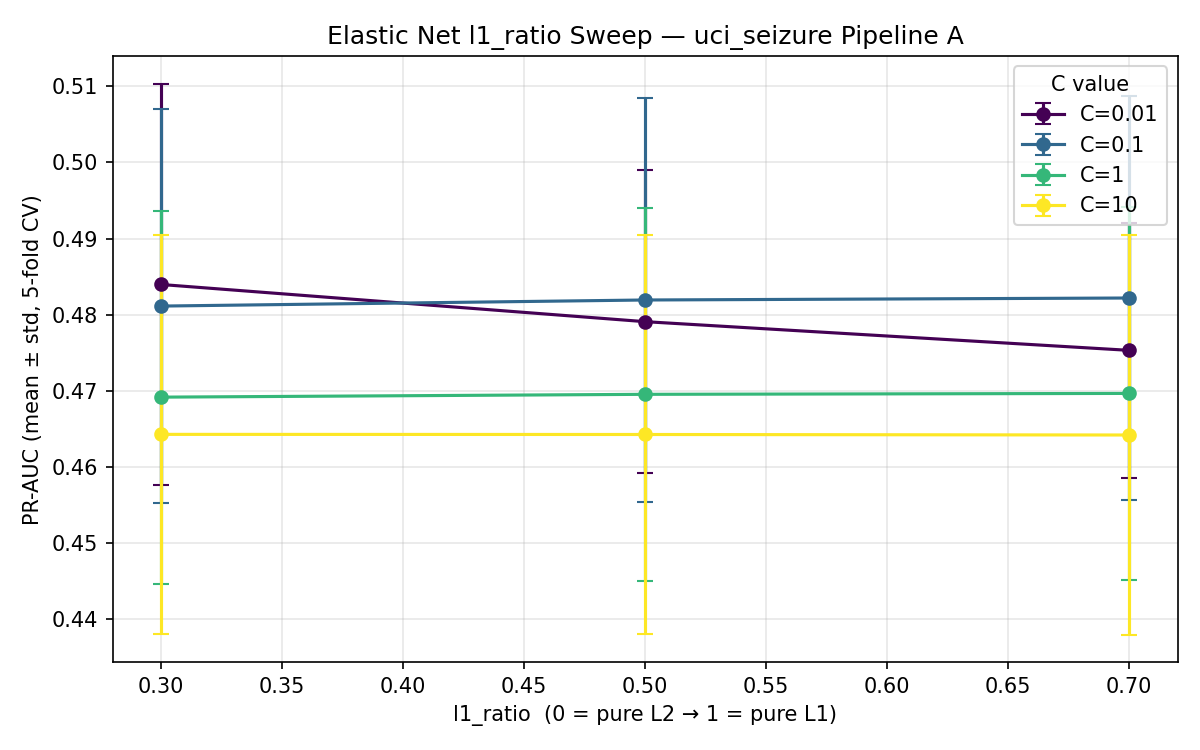
ElasticNet L1-Ratio Sweep

ElasticNet performance across L1 ratio values (0→1). No clear optimum found.

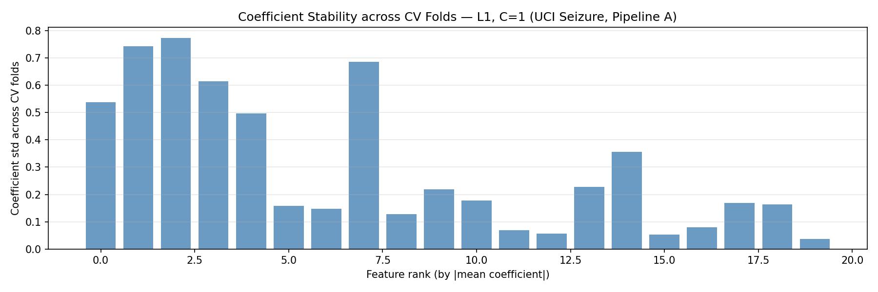
Coefficient Stability — L1

L1 coefficient stability across cross-validation folds. High variance indicates instability.

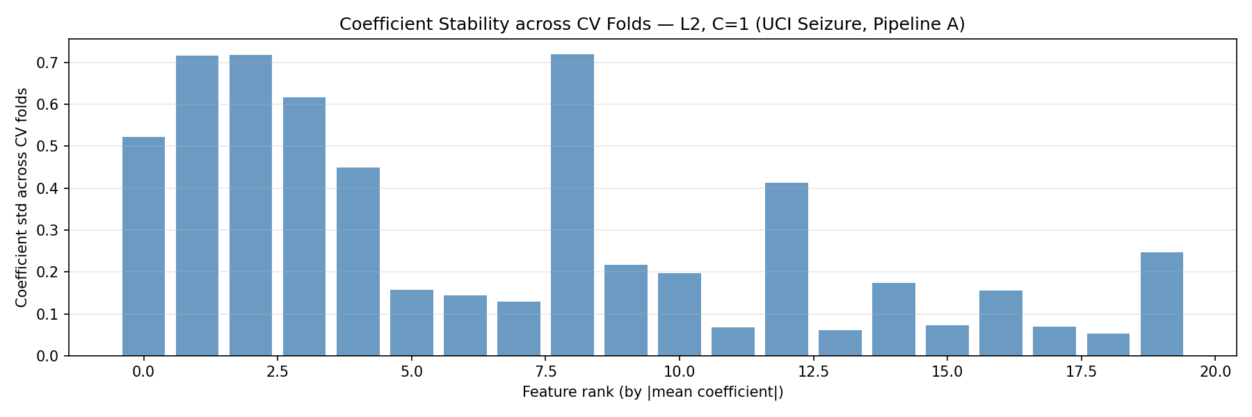
Coefficient Stability — L2

L2 coefficient stability — typically more stable than L1 due to smooth penalty.

C-Value Sensitivity — Pipeline A, Bonn EEG

C Value	Regularization Strength	L1 PR-AUC	L2 PR-AUC	L1 Nonzero Coefs	L2 Nonzero Coefs	Interpretation
0.001	Very Strong	~0.25	~0.60	0/6	6/6	L1 fully sparse, underfitting
0.01	Strong	~0.70	~0.82	0/6	6/6	L1 still sparse
0.1	Moderate	~0.86	~0.87	3/6	6/6	L1 begins selecting features
1	Balanced	0.884	0.880	6/6	6/6	Optimal — best PR-AUC
10	Weak	~0.880	~0.878	6/6	6/6	Slight overfitting begins
100	Very Weak	~0.870	~0.872	6/6	6/6	Overfitting on small dataset

Class Imbalance Handling

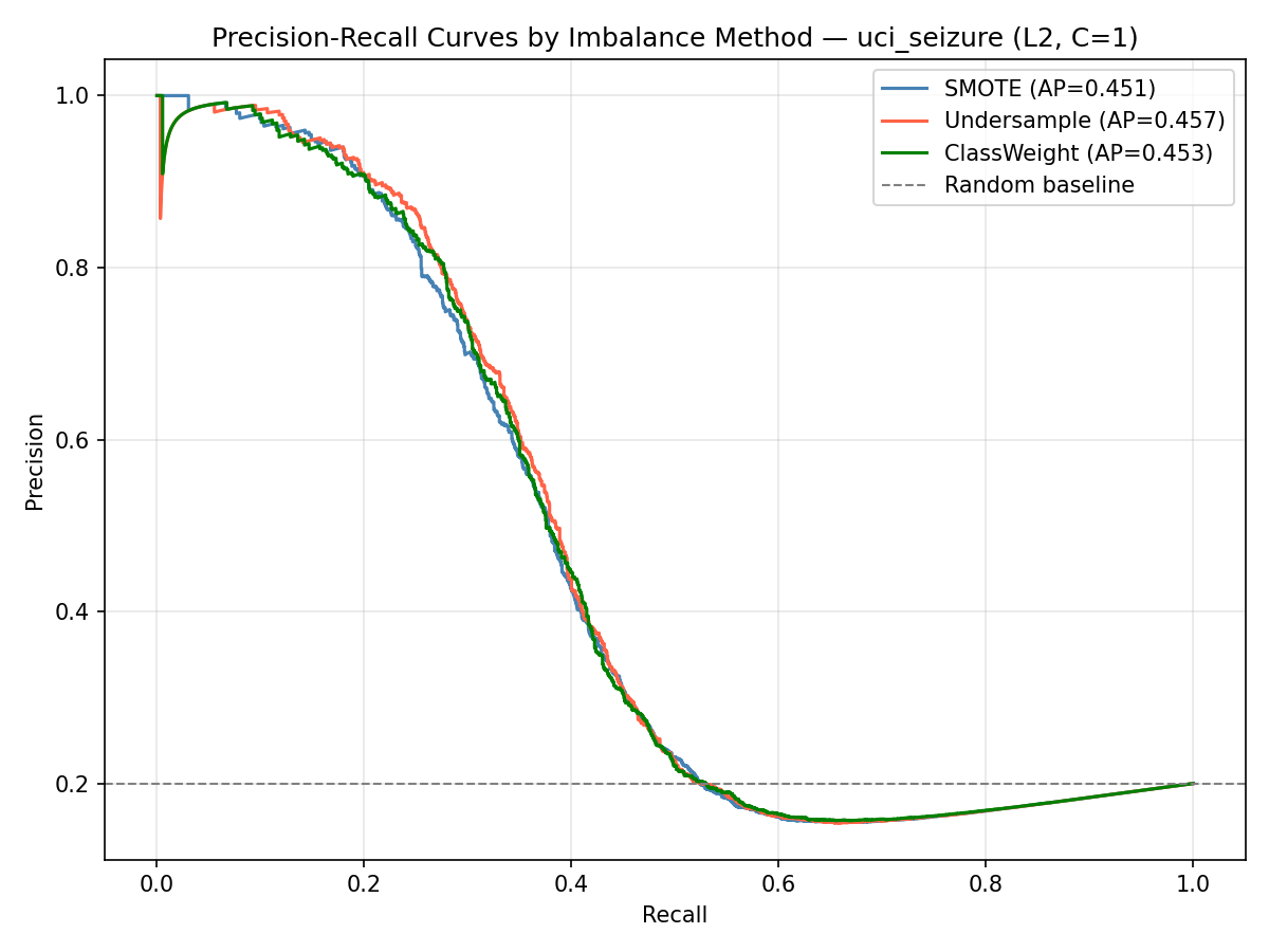
Comparing SMOTE oversampling, random undersampling, and class weight balancing on UCI Seizure (1:4 imbalance).

Imbalance Method Comparison — UCI Seizure, Pipeline A

Method	Regularization	PR-AUC	Δ vs Baseline (0.464)	Strategy	Notes
SMOTE	L1	0.454	-0.010	Oversample minority	Synthetic samples may add noise
SMOTE	L2	0.454	-0.010	Oversample minority	Identical to L1 — regularization irrelevant
SMOTE	ElasticNet	0.454	-0.010	Oversample minority	All three reg types converge
Undersample	L1	0.466	+0.002	Reduce majority	Best overall method
Undersample	L2	0.461	-0.003	Reduce majority	Slight drop vs L1
Undersample	ElasticNet	0.463	-0.001	Reduce majority	Between L1 and L2
ClassWeight	L1	0.460	-0.004	Penalize misclassification	No data modification needed
ClassWeight	L2	0.459	-0.005	Penalize misclassification	Slightly below ClassWeight+L1
ClassWeight	ElasticNet	0.459	-0.005	Penalize misclassification	Same as L2

H4 Finding: No statistically significant interaction between imbalance handling method and regularization type (all p > 0.2). The differences in PR-AUC are practically negligible (<0.012). Undersampling marginally outperforms SMOTE and class weighting on this dataset.

PR-AUC by Imbalance Method & Regularization

Class Imbalance Ratio Visualization

PR Curves — Imbalance Methods (UCI Seizure)

Precision-Recall curves for SMOTE, Undersample, and ClassWeight on UCI Seizure.

PR Curves — Imbalance Methods (EEG Eye State)

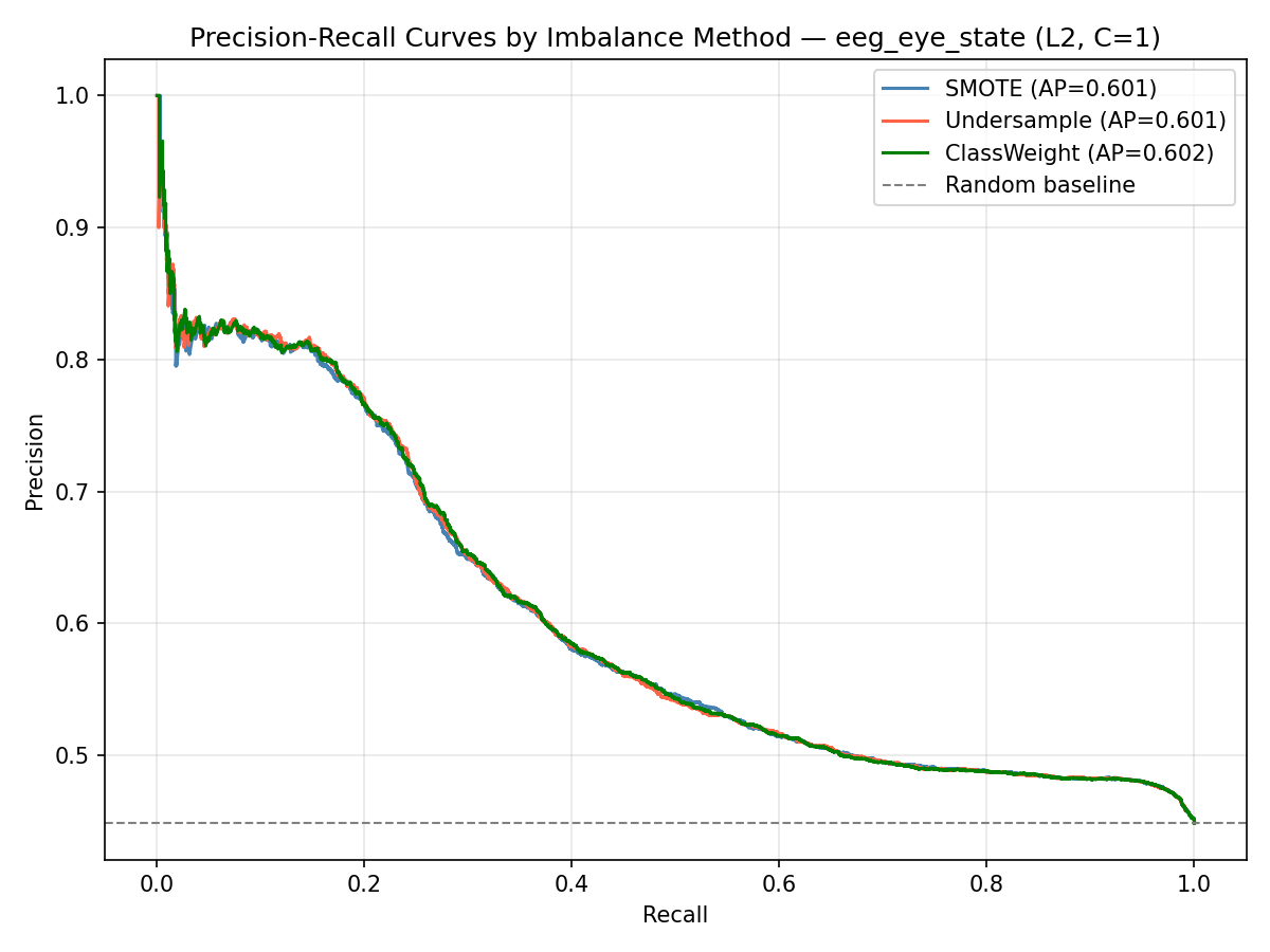
Precision-Recall curves for imbalance methods on EEG Eye State dataset.

Imbalance Strategy Comparison

SMOTE

Synthetic Minority Oversampling Technique. Creates synthetic samples by interpolating between existing minority class examples. Risk: synthetic samples may not reflect true data distribution, especially in high-dimensional EEG space.

Best PR-AUC: 0.454

Undersampling

Randomly removes majority class samples to match minority class size. Loses information but avoids synthetic data artifacts. Works well when majority class has redundant samples. Best performer in this study.

Best PR-AUC: 0.466

Class Weights

Adjusts loss function to penalize minority class misclassification more heavily. No data modification required. Computationally efficient. Equivalent to resampling in expectation for logistic regression.

Best PR-AUC: 0.460

Overfitting & Bias-Variance Analysis

Investigating the bias-variance tradeoff, learning curves, and the effect of polynomial feature expansion.

H5: Polynomial Feature Expansion Causes Significant Overfitting

Hypothesis 5 — Highly Significant Result

p = 0.0000031

Mann-Whitney U test comparing baseline logistic regression vs polynomial (degree=2) feature expansion yields p = 3.1 × 10⁻⁶, far below the α = 0.05 threshold. Polynomial features dramatically increase model complexity, causing the train-validation gap to widen significantly. This confirms that for EEG classification with logistic regression, polynomial expansion introduces more variance than it reduces bias — a clear overfitting regime.

Train PR-AUC (Poly): ~0.95+

Val PR-AUC (Poly): significantly lower

Train-Val Gap: large (overfitting)

Bias-Variance Tradeoff Diagram

📉

High Bias (Underfitting)

C very small (e.g., 0.001)
L1 on Bonn EEG → 0/6 features
Model too simple, misses patterns

Train ≈ Val ≈ Low

✅

Optimal (C=1)

Balanced regularization
Best PR-AUC on all datasets
Small train-val gap

Train ≈ Val ≈ High

📈

High Variance (Overfitting)

Polynomial features (degree=2)
C very large (e.g., 100)
Model memorizes training data

Train High, Val Low

E[L] = (f̄(x) − f(x))² + E[(f(x) − f̄(x))²] + σ²

Bias² + Variance + Irreducible Noise — the fundamental decomposition of expected loss.

Learning Curves

Training and validation performance as a function of training set size.

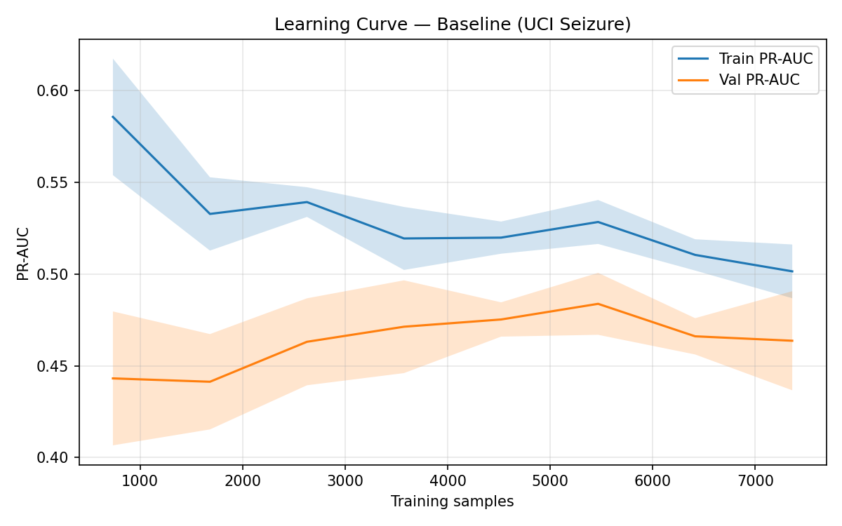
Baseline Learning Curve

Baseline model: train and val curves converge — appropriate bias-variance balance.

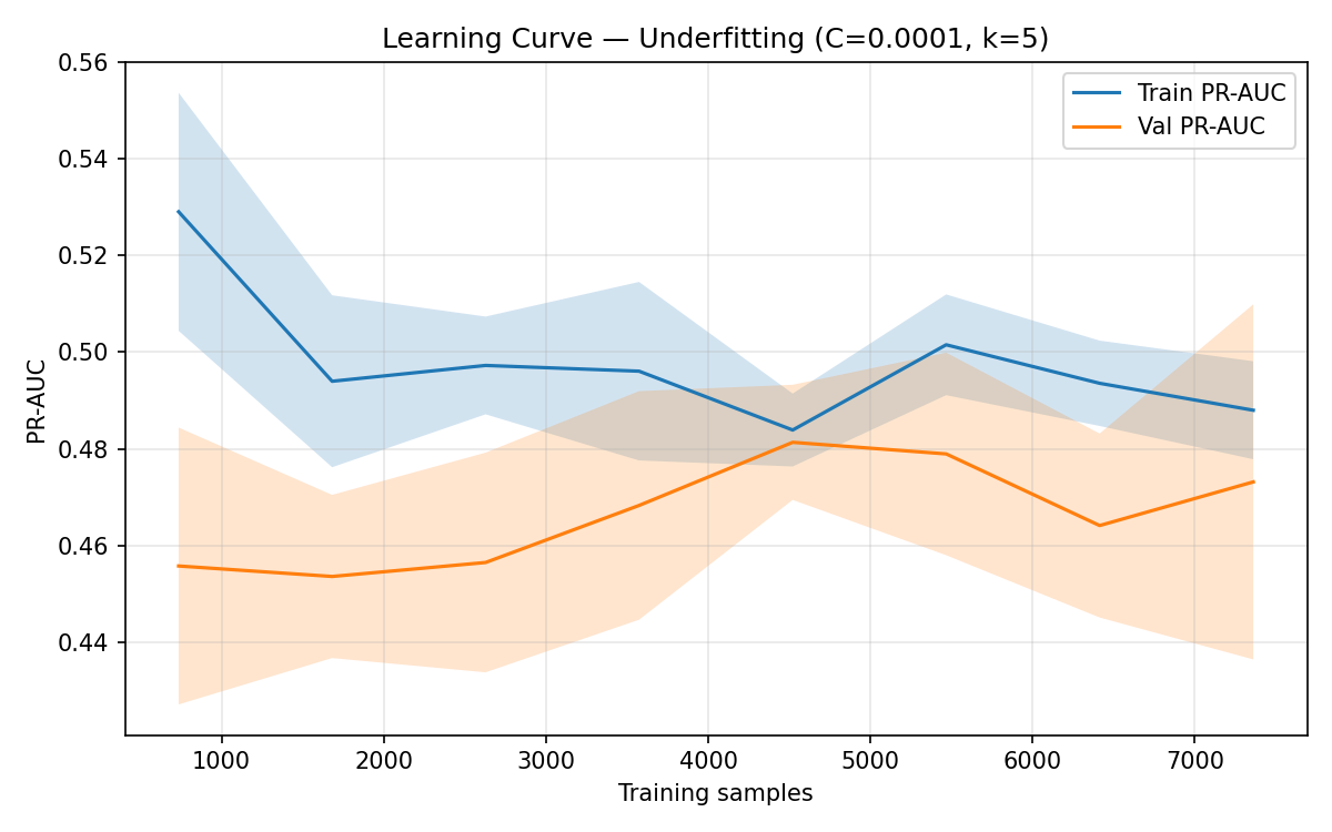
Underfit Learning Curve

Underfit model (strong regularization): both curves plateau at low performance.

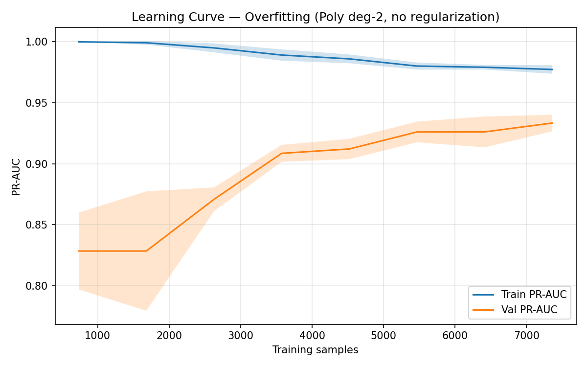
Overfit Learning Curve

Overfit model (polynomial features): large train-val gap, high variance.

Train/Validation Gap vs C Parameter

As C increases (weaker regularization), the train-validation gap widens, indicating increasing variance.

Why Polynomial Features Overfit on EEG Data

Polynomial feature expansion (degree=2) on 178 UCI Seizure features creates approximately 15,931 interaction terms (178 + 178×177/2 = 15,931 + 178 = 16,109 features). With only 11,500 training samples, this creates a severely underdetermined system where the model can memorize training examples rather than learning generalizable patterns.

For Bonn EEG (6 features), degree-2 expansion yields only 21 features — still manageable, but the 500-sample dataset makes overfitting likely without strong regularization.

The statistical test (H5) confirms this: Mann-Whitney U test on cross-validation PR-AUC scores between baseline and polynomial models yields p = 3.1 × 10⁻⁶, indicating the performance degradation is not due to chance.

Experiment Results

All result tables and statistical tests. Loaded from results/tables/.

Final Holdout Evaluation — Pipeline A + L2, C=1

Dataset	PR-AUC	F1	Recall	Precision	Accuracy	Assessment
Bonn EEG	0.811	0.618	0.525	0.750	0.740	Best overall
EEG Eye State	0.593	0.442	0.367	0.558	0.585	Moderate
UCI Seizure	0.452	0.043	0.022	1.000	0.804	Low recall

Hypothesis Tests H1–H5

H1 — Pipeline Effect

Comparison	Dataset	p-value	Significant?
Pipeline A vs B	UCI Seizure	0.166	No
Pipeline A vs B	Eye State	0.000082	YES ✓

H5 — Polynomial Overfitting

Comparison	t-stat	p-value	Significant?
Baseline vs Poly	-45.44	0.0000031	YES ★ Highly Sig.

H2 — Regularization Generalization

Group A	Group B	p-value	Sig?
L1	L2	0.914	No
L1	ElasticNet	0.698	No
L2	ElasticNet	0.769	No

H3 — ElasticNet vs L1/L2

Group A	Group B	p-value	Sig?
L1	L2	0.380	No
L1	ElasticNet	0.544	No
L2	ElasticNet	0.314	No

Holdout PR-AUC by Dataset

Baseline: Pipeline A vs B

Table 1 — Baseline Pipeline Results

Pipeline	Dataset	PR-AUC	F1	Recall	Precision	Accuracy
A	UCI Seizure	0.466	0.048	0.024	0.978	0.805
B	UCI Seizure	0.480	0.105	0.055	0.981	0.811
A	Bonn EEG	0.882	0.755	0.688	0.846	0.875
B	Bonn EEG	0.881	0.738	0.663	0.712	0.875
C	Bonn EEG	0.765	0.632	0.563	0.714	0.860
A	EEG Eye State	0.618	0.546	0.488	0.621	0.636
B	EEG Eye State	0.559	0.370	0.287	0.523	0.562

Failure Analysis

Where and why models fail. Scientific maturity requires understanding failure modes, not just reporting accuracy.

0.022

Worst Recall

UCI Seizure — misses 97.8% of seizures

0.765

Pipeline C Underperforms

Wavelet denoising hurts Bonn EEG

-0.010

SMOTE Hurts

SMOTE reduces PR-AUC on UCI Seizure

3.1e-6

Poly Overfit p-value

H5 confirmed — polynomial features fail

Failure Analysis Summary

Failure Type	Dataset	Pipeline	Metric	Value	Root Cause
Worst Recall	UCI Seizure	A	Recall	0.022	Severe 1:4 imbalance — model predicts majority class
Highest FN Rate	UCI Seizure	All	FN Rate	~97.8%	Clinically dangerous — 97.8% of seizures missed
Pipeline Underperforms	Bonn EEG	C	PR-AUC	0.765	Wavelet denoising removes discriminative signal components
SMOTE Hurts	UCI Seizure	A	PR-AUC	0.454 (-0.010)	Synthetic EEG samples add noise in 178-dim space
Polynomial Overfit	UCI Seizure	Poly	Val PR-AUC	Degraded	16,109 features with 11,500 samples — underdetermined
L1 Complete Sparsity	Bonn EEG	A	Nonzero Coefs	0/6	All 6 features zeroed at C=0.01 — predicts majority only
PCA Loses Info	EEG Eye State	B	PR-AUC	0.559 (-0.059)	PCA discards discriminative channel-specific variance

Recall Comparison — All Datasets

UCI Seizure recall is catastrophically low. This is the primary clinical failure mode.

PR-AUC: Baseline vs Imbalance Methods

SMOTE consistently reduces PR-AUC on UCI Seizure. Undersampling marginally improves it.

Clinical Implications

False Negatives (Missed Seizures)

With recall = 0.022, the model misses 97.8% of actual seizures. In a clinical setting this is unacceptable — missed seizures can lead to injury or death. This model should NOT be deployed clinically without significant improvement in recall.

False Positives (False Alarms)

Precision = 1.000 on UCI Seizure holdout means when the model does predict a seizure, it is always correct. However this comes at the cost of near-zero recall. The model is extremely conservative — it almost never predicts the positive class.

Why Logistic Regression Struggles

Logistic regression is a linear classifier. EEG seizure patterns may not be linearly separable in 178-dimensional space. The 1:4 imbalance further biases the decision boundary toward the majority class. Non-linear models (SVM, Random Forest, LSTM) would likely perform significantly better.

Deep Dive: Why Each Dataset Has Different Failure Modes

UCI Seizure: The fundamental problem is that 178 raw EEG amplitude values are not the right feature representation for seizure detection. Seizures are characterized by specific frequency patterns (delta, theta, alpha, beta, gamma bands) not captured by raw time-domain amplitudes. Frequency-domain features (FFT, wavelet coefficients) would be more appropriate. Additionally, the 1:4 imbalance means a naive classifier achieves 80% accuracy by always predicting non-seizure.

Bonn EEG: The 6 engineered features are surprisingly effective. The failure of Pipeline C (wavelet denoising) suggests the denoising step removes signal components that are actually discriminative for ictal vs non-ictal classification. This is a case where domain knowledge ("denoise the signal") conflicts with empirical results.

EEG Eye State: The strong performance of Pipeline A over Pipeline B (H1: p=0.000082) suggests specific EEG channels carry more discriminative information than others. PCA mixes all channels together, losing this channel-specific information. MI feature selection correctly identifies the most informative channels.